
Playing with Computational Physics
At some point during the process of working through my dissertation, I got so bogged down in the process of doing the work, I forgot a bit why I was so intrigued when I started. I was going through the motions, but not really finding the fun of physics. Sure, programming is fun in and of itself, but I was missing the physics. So, now that I have free time to pursue a hobby, I want to go back and remind myself why I started down this path.
So, where to go? I am one of those people who value a good book. And I do mean a physical book. I bought and kept all of my text books throughout my undergrad and graduate work. That being the case, I grabbed my undergraduate computational physics book by Nicholas J. Giordano and Hisao Nakanishi [1] and decided to work through it again. It is a fantastic book that covers a broad span of topics with many fun problems that I can play with.
With that all said, I plan on working through all of the problems starting at the beginning. I will periodically post a selection of the discussion of the solutions here, but some problems are trivial and don’t merit much in the way of discussion. I will be working with Python primarily, but I may dust of my Fortran skills for some of the problems. I will also be attempting to keep the code recognizable and avoid clever tricks like list comprehensions in the physics parts. It’s not that I don’t know them (I do), I’m just trying to keep to the basics. Anything to do with display or I/O is fair game though. The code will be hosted in a mercurial repository on Bitbucket. Why Bitbucket and mercurial [f1] you ask? Because it’s Python.
And now for a final note before I get started. If you are an undergraduate using this text, go do your homework before looking over my solutions. It’s good for you and actually quite fun.
Chapter 1
And so it begins. This will probably be a very short section because the problems are very simple. The chapter is simply a chance to whet the appetite and brush up on some basics. It will also give me a chance to build some basic plotting tools for later.
Problem 1
Not much to see here. It is pretty trivial to see that the solution is \(v(t) = v(0) - g t\). Each time step is similarly simple \(t_i = i \Delta t\). Computing over a selection of time steps, we find

Numeric and exact solution for chapter 1 problem 1.
Well, that’s not very interesting. It is good to know that we can get a good answer for this case, but what about the error?

Error in the solution for chapter 1 problem 1.
Now, that’s more interesting. What are the final results? I’m glad you asked:
Numeric |
Exact |
Difference |
-98.000000 |
-98.000000 |
-7.95808e-13 |
-98.000000 |
-98.000000 |
-2.70006e-13 |
-98.000000 |
-98.000000 |
4.26326e-14 |
-98.000000 |
-98.000000 |
2.84217e-14 |
-98.000000 |
-98.000000 |
-1.42109e-14 |
-98.000000 |
-98.000000 |
0 |
We clearly see that increasing the time step decreases the error. This is contrary to the common result where decreasing the time step increases the accuracy. What’s going on here? The answer is accumulated error due to machine precision. At each time step, we are accumulating a fractional error. As we take more steps from the start to the finish, we are simply adding up all that error. Tricks exist that you can use to reduce the error, but they use fancy array slicing which I am avoiding.
Problem 2
Not much to see here, unless you didn’t do problem 1. Then it’s the exact same as above but with an opposite sign. The accuracy is better, but I suspect that is due to a nice multiple of 10.
Problem 3
Now we get to something non-trivial. Implementing the Euler method is straight forward. At some point, I will probably need to write a canned routine to perform the Euler method, but that seems to be touching on the area I want to avoid. We’ll see. But now results. Plotting for a selection of \(b\), we see that the terminal velocity is being reached as expected. A bit of manipulation reveals that terminal velocity is when \(v_t = a / b\) which is what we are seeing. Beyond that, there isn’t really much more to say. I know we’ll come back to this in the next chapter.

Numeric and exact solution for chapter 1 problem 3.
Problem 4
And now we get to the first “challenging” problem. Coding up the numerical solution is straight forward. The real challenge is in finding the analytic solution, and I must say, I have been out of ordinary differential equations for so long that it stumped me. My first attempt was guess and check. That failed horribly. Then, I attempted to use a power series expansion. That also failed. The correct method was to use a trial function.
We begin with the set of equations
where \(u = t / \tau_A\) and we define \(R \equiv \tau_A / \tau_B\). The solution to the first equation is trivial
The second equation is the trickier part. First, move \(N_B\) to the left hand side and multiply by \(e^{Ru}\)
(Quick aside: apparently, both Jekyll and MathJax strip a backslash. Meaning, to get that line break above I had to use \\\\.) Integrating both sides we find
Now, if we have a population \(N_B(0)\) at time \(u=0\), we can solve for \(C\) to find \(C = N_B(0) - \frac{N_A(0)}{R-1}\). Putting it all together, we find
But wait, there’s more! We clearly see a special case when \(\tau_A = \tau_b\). Then \(R=1\) the solution is a bit different. In this case, we have
Plugging in the stated initial conditions we have
Now we get to see what happens. Below, I present a batch of plots. In each cell, the top figure plots the numeric and exact results for \(N_A(u)\) and \(N_B(u)\) with \(u=t/\tau_A\). The bottom plot in each cell is the error at each time step. All figure share a common X-axis and each row shares a Y-axis. From left to right, we are reducing the time step and increasing the number of iterations in the simulation. Going down the column, we are increasing the ratio of the time constants \(R\equiv \tau_A/\tau_B\).
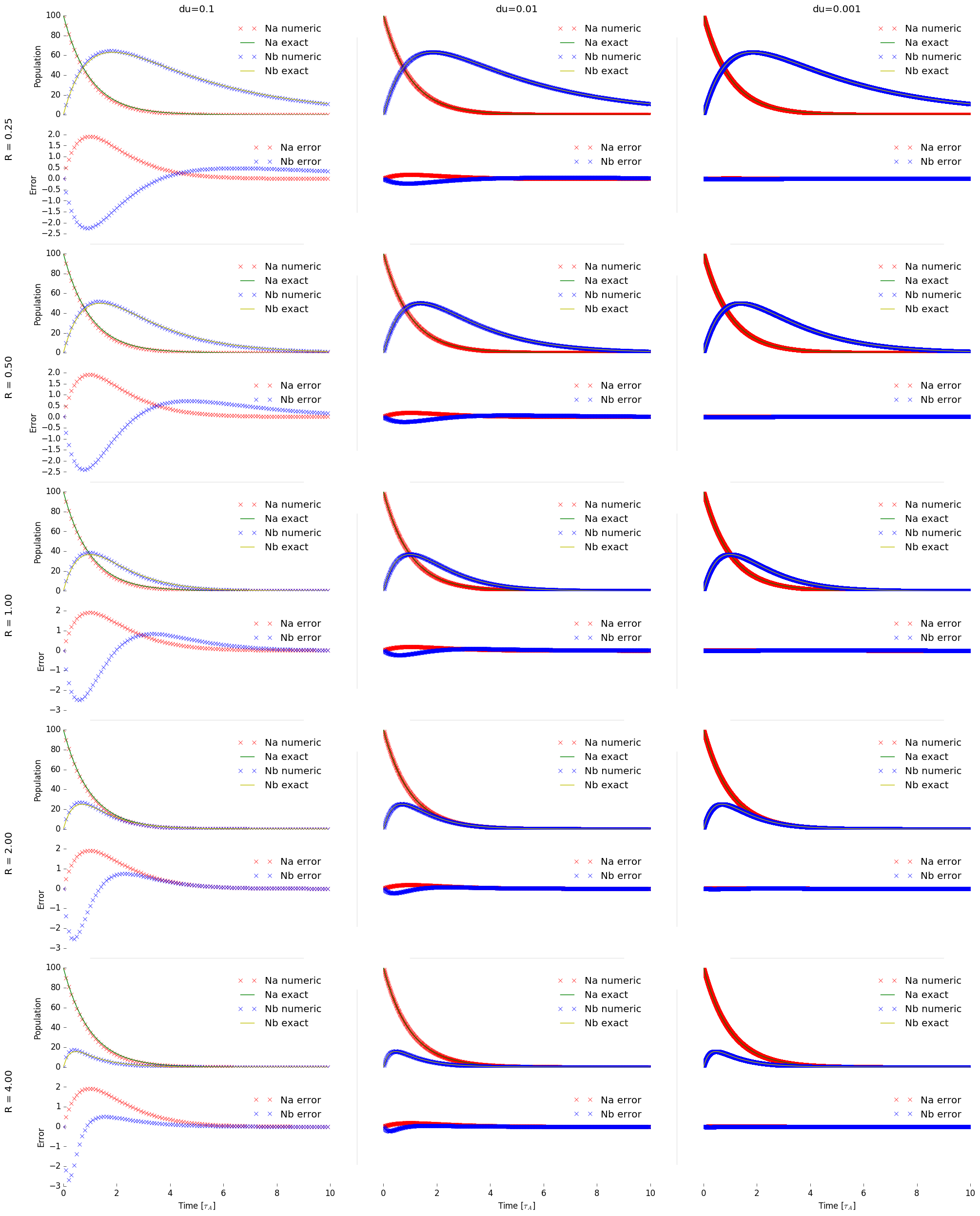
Numerical and exact solutions for chapter 1 problem 4.
The first thing that jumps out to me is that the error is fairly stable with respect to \(R\). It does increase with a larger time constant ratio, but it is not as large as one might expect. We see that using a time step of \(\Delta u = 0.001\) yields fairly accurate results for all cases. We could increase the accuracy by increasing the number of iterations, but I got impatient and killed the calculation. We have more interesting things to do!
Generally speaking, we see that the population \(N_B\) has a form similar to the Planck blackbody curve. A quick glance at the equations does not really reveal an specific relation. I suspect that this is just a random occurrence. Many equations in physics that bear a superficial similarity. We also see that when \(N_A\) decays faster than \(N_B\), we get a strong surge in the population of \(N_B\). This is true when both decay at the same rate as well. I’m sure as I stare at this figure some more, I will come up with other things to say. But for now, I’m calling it quits. Oh, and for estimating the short and long term behavior, after looking at the graphs it’s trivially easy. There is a power law increase in \(N_B\) and power law decrease in \(N_A\) at the early times followed by an exponential decay at long times.
Problem 5
And on to the next challenging problem. First and foremost, we don’t need to go for the simplicity stated in the problem. We can keep our solution general and play around with the ratio of time constants. The first thing we need to do is recast the problem to remove the units. To do this, we introduce the ratio of time constant \(R=\tau_A/\tau_B\) as in the previous problem. This in turn transforms our problem int the set of equations
where \(f\) is the population of A and \(g\) is the population of B. This is mainly to save me some typing. Now we can turn this system of equations over to a mathematician and get an answer!
Now for a brief aside about removing the units. In the above equation, we are working with a scaled time parameter \(u=t/\tau_A\) and the time constant ratio \(R\). One thing my first quantum mechanics professor pointed out is that you always want to work with unitless variables. The scale factors you find turn out to be very important in determining relative properties of the problem. He mentioned this while we were studying the simple harmonic oscillator system. There, the solution can be studied in a general sense simply with \(x_0\) and \(p_0\). The net result is the units are where the physics exists.
Before we get to the numeric solution, we can actually find an analytic solution to these equations. We don’t really need it for the problem, but it is good to evaluate the error in out solution. Also, it gives me a chance to brush up on my differential equations. First, we write \(f\) in terms of \(g\) and take the derivative
Now we introduce our proposed solution \(g = e^{mu}\) and plug it in. This gives us the equation
with the solutions \(m=0\) and \(m=-R-1\). Taking a linear combination of the two solutions we find
Now, if we take \(f(0) = A\) and \(g(0) = B\), we can plug these in to find
(The algebra isn’t that hard if you really want to work through it.) Adding these two solutions readily shows that the population at any time is \(f+g = A+B\) as expected. Additionally, we can see the long term behavior should be
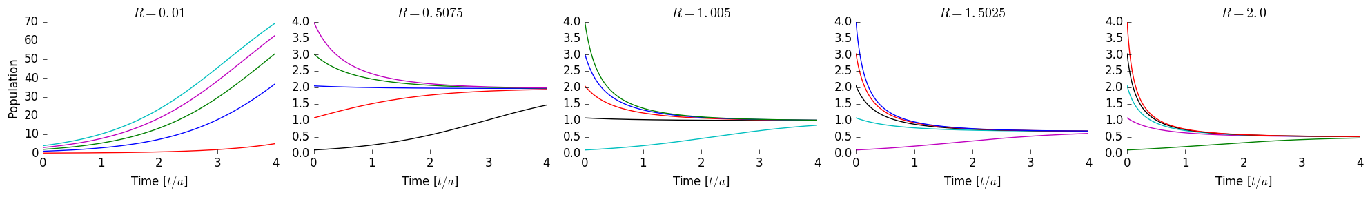
So, if the time constants are equal, we get equal populations in both states. On the other hand, if population A decays slower than B (\(R > 1\)), we will have a larger population is A than B. We have no real reason to consider the case where A decays faster than B because we can simply get that by swapping the two states. Now that we have the theory and math done, let’s write some code.
Well, that took longer than it should have. The main reason was I was trying to generate a figure with the number of steps I was using for the number of rows and not the number of populations. Lesson: Always make sure you’re using the correct parameters. Stupid mistake…
On to the show! First, we consider when the ratio of the time constants is the same \(R=1\). Playing around with the number of steps, I found 10000 to work just fine. The error is proportional to the number of steps. Doubling the number of steps used halves the error. Below, I present the population, derivative of the population, and the error in each column.
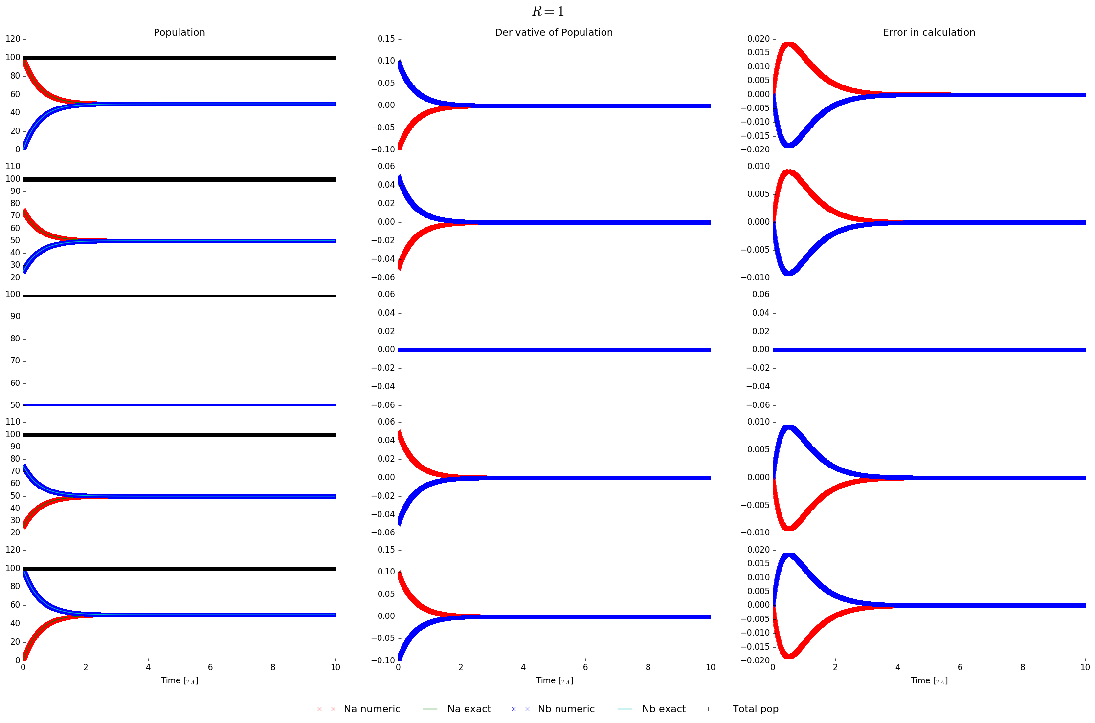
Numerical and exact solutions for chapter 1 problem 5.
Looking at this, we see that the result is boring. The two states decay into a state where they are exchanging member equally. Normally, I would propose looking at the others, but the result is the same. Those systems just end at a different population distribution governed by the ratio \(R\). We do see that the numerical value of the derivative goes to zero as expected. Unfortunately, this problem only gave me an exercise in debugging and creating plots. Time to move on.
Problem 6
And now on to the final problem of the chapter. First off, performing the exercise of error analysis using the \(b=0\) case is pointless. It is simply exponential growth, and we did that analysis for problems 1 and 2. Now for a figure:
Numerical and exact solutions for chapter 1 problem 6.
Looking at this, we see that the long term behavior of the population is to converge to the value \(N=a/b\). This can be verified as the expected behavior from the outset by setting the derivative to 0 and solving for the population. To further the analogy to a population, we see that the population will grow until it maximizes the resources available. At that point, the population cannot sustain additional growth without losing members. On the other hand, if the population exceeds its resources, the limited supply will force members out until the resources can sustain the remaining population.
Conclusion
With that said, we have reached the end of chapter 1. Looking at this post, I see that it got rather long. To that end, I will start by breaking the chapters into individual posts. At some point in the near future, I will get to work on chapter 2.
Note
Taking another look at these figures while migrating my website, I see a major error that I admonish both my colleagues and students about: The figures are not crafted for the target space. Notice how hard it is to read the labels. This is indicative of not paying attention to how the figure will be used (i.e. relying on scaling to make the figure fit). If the target width is 5 in., then tell your plotting utility to generate a 5 in. figure. If the space is 500 px, then use 500 px and set the fonts correctly. If your plotting utility cannot do this, get a better plotting utility.